This is an experimental first post in physics. I somehow made it resemble a textbook or a classroom note too much. I am not sure if this is the final form I want, but I did spend a fair amount of time making this post—whatever improvements there are, I will make them next time (topic not decided yet).

References: Spacetime and Geometry (Sean Carroll); Black Holes, White Dwarfs, and Neutron Stars (Stuart L. Shapiro & Saul A. Teukolsky); “Nonradial instabilities in anisotropic neutron stars” (Shu Yan Lau et al.).

Lie Derivative and Fluids

This post serves as a concise note with necessary derivations to understand perturbation in fluids. One would find it useful when modeling stars, their EOS, or stability, as one treats the stellar interior as fluid units, and for a single unit, one only cares about its bulk properties. The reason Lie derivative is included is that, with the presence of a gravitational field, the spacetime metric where the fluid resides may no longer be Minkowski. We therefore need to treat it with techniques in differential geometry.

I plan to first introduce the necessary background to understand and calculate the Lie derivative on a manifold, and then summarize its applications when modeling fluids. The last section consists of a short example of calculating a perturbed stress-energy tensor.

Manifold Maps, Pullback and Pushforward

A more detailed version of this section can be found in Appendix A & B of Sean Carroll’s Spacetime and Geometry.

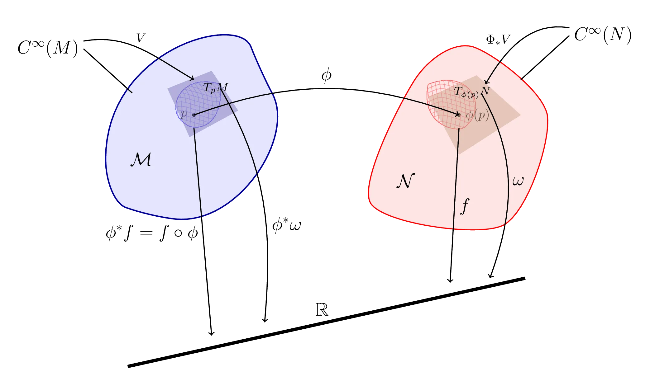
We start with manifolds $M$ and $N$, with dimensions $m$ and $n$, and the function $\phi$ is a map from $M\to N$ and function $f$ is a map from $N\to \mathbb{R}$.

One is able to define the Pullback of $f$ by $\phi$, denoted by $\phi^* f:=(f\circ \phi)$ We can think of it as pulling back the function $f$ from $N$ to $M$. We however cannot push the function forward, but despite this, since we can see vectors as derivative operators that maps smooth functions to real numbers, we can define the Pushforward of a vector. Suppose V(p) is a vector at point $p$ on $M$, the pushforward vector $\phi_*V$ at the point $\phi(p)$ on $N$ by giving its action on $N$: $(\phi_*V)(f) := V(\phi^* f)$

With $V^\mu$ being the coefficients and $\partial_\mu = \partial/\partial x^\mu$, $\partial_\alpha = \partial/\partial x^\alpha$ being the basis of $V$ on $M, N$ respectively, we have: $V(\phi^* f) = V^\mu\partial_\mu(f\circ\phi) = V^\mu \frac{\partial y^\alpha}{\partial x^\mu}(\partial_\alpha f)$ It resembles the change of coordinate but note that $\alpha$ and $\mu$ can take different values, meaning there is no reason for the “Jacobian Matrix” $\partial y^\alpha/\partial x^\mu$ to be invertible.

Similar to the pushforward of a vector, one can also define the pullback of a oneform $\omega$: $(\phi^*\omega)(V) := \omega (\phi_* V) = \frac{\partial y^\alpha}{\partial x^\mu} \omega_\alpha V^\mu$

One can think the way below to have an intuition :

$$\begin{aligned} V:\,& C^\infty(M) \to T_pM&\\ \phi^*V:\,& C^\infty(N) \to T_pN\\ \omega:\,&T_pM\to \mathbb{R} \\ \phi_*\omega:\,& T_pN \to \mathbb{R} \end{aligned}$$

One can extend fullback and pushforward to arbitrary $(0,l)$ or $(k,0)$ tensors respectively:

$$\begin{aligned} (\phi^* T)_{\mu_1\cdots \mu_l} =& \frac{\partial y^{\alpha_1}}{\partial x^{\mu_1}}\cdots\frac{\partial y^{\alpha_l}}{\partial x^{\mu_l}}T_{\alpha_1\cdots \alpha_l}\\ (\phi^* S)^{\alpha_1\cdots \alpha_k} =& \frac{\partial y^{\alpha_1}}{\partial x^{\mu_1}}\cdots\frac{\partial y^{\alpha_k}}{\partial x^{\mu_k}}S^{\mu_1\cdots \mu_k} \end{aligned}$$

Lie Derivatives

We need the definition of a diffeomorphism to further the discussion. From the previous section we have defined pullback and pushforward with the map $\phi$, however, in most case $\phi$ cannot work both ways since it’s not invertible.

Now we set $M$ and $N$ to be the same manifold, automatically meaning they are diffeomorphic: there exist a smooth map $\phi : M\to N$ with a smooth inverse $\phi^{-1} : N\to M$. We can now pullback or pushforward arbitrary tensors:

$${(\phi^* T)^{\alpha_1\cdots \alpha_k}}_{\beta_1\cdots\beta_l} = \bigg(\frac{\partial y^{\alpha_1}}{\partial x^{\mu_1}}\cdots\frac{\partial y^{\alpha_l}}{\partial x^{\mu_l}} \bigg)\bigg(\frac{\partial y^{\nu_1}}{\partial x^{\beta_1}}\cdots\frac{\partial y^{\nu_l}}{\partial x^{\beta_l}}\bigg){T^{\mu_1\cdots \mu_k}}_{\nu_1\cdots\nu_l}$$

In this setup, diffeomorphisms and coordinate transforms are simply two different ways of doing the exact same thing.

---

Given a diffeomorphism $\phi:M\to M$ and a tensor field ${T^{\mu_1\cdots \mu_k}}_{\nu_1\cdots\nu_l}(x)$, we can now compare the value of the tensor at $p$ and $\phi^*\left[{T^{\mu_1\cdots \mu_k}}_{\nu_1\cdots\nu_l}(\phi(p))\right]$, the value of the tensor at $\phi(p)$ pulled back to $p$. This allows us to define another kind of derivative on manifolds - one that characterizes the change of tensor quantities as they move along the flow of the diffeomorphism. However, we need further restrict the diffeomorphism to a one-parameter family of diffeomorphisms $\phi_t$, which can be thought of as a smooth map $\mathbb{R}\times M\to M$, such that for each $t\in \mathbb{R}$ there is a diffeomorphism $\phi_t$, satisfying $\phi_s\circ \phi_t = \phi_{s+t}$. A very intuitive such diffeomorphism is given by $\phi_t(\theta,\phi) = (\theta,\phi+t)$ on $S^2$.

One can also reverse construct to define such one-parameter family of diffeomorphisms from a given vector field: suppose there is a vector field $V^\mu(x)$, then the integral curves of the vector field is chosen to be the curves $x^\mu(t)$ that solve: $\frac{dx^\mu}{dt} = V^\mu$ The vector field is called the generator of the diffeomorphism.

The Lie derivative of the tensor along the vector field is given by:

$$\begin{aligned} \mathcal{L}_V{T^{\mu_1\cdots \mu_k}}_{\nu_1\cdots\nu_l} :=&\lim_{t\to 0}\bigg(\frac{\Delta_t{T^{\mu_1\cdots \mu_k}}_{\nu_1\cdots\nu_l}}{t}\bigg)\\ =&\lim_{t\to 0}\bigg(\frac{\phi_t^*[{T^{\mu_1\cdots \mu_k}-}_{\nu_1\cdots\nu_l}(\phi_t(p))]-{T^{\mu_1\cdots \mu_k}}_{\nu_1\cdots\nu_l}}{t}\bigg) \end{aligned}$$

The operator $\mathcal{L}_V$ is linear and obeys Leibniz rule. It is a more primitive notion than the covariant derivative as it does not require a connection, and it reduces to the ordinary directional derivative on functions. Meanwhile, when calculating the Lie derivative of a scalar field, the result reduces to the action of the vector field itself acting on the scalar field.

$$\mathcal{L}_V\Phi = V^\mu\partial_\mu\Phi$$

And a general form of the Lie derivative takes the form:

$$\begin{aligned} \mathcal{L}_V T^{\mu_1 \mu_2 \cdots \mu_k}_{\nu_1 \nu_2 \cdots \nu_l} &= V^\sigma \partial_\sigma T^{\mu_1 \mu_2 \cdots \mu_k}_{\nu_1 \nu_2 \cdots \nu_l} \\ &\quad - (\partial_\lambda V^{\mu_1}) T^{\lambda \mu_2 \cdots \mu_k}_{\nu_1 \nu_2 \cdots \nu_l} - (\partial_\lambda V^{\mu_2}) T^{\mu_1 \lambda \cdots \mu_k}_{\nu_1 \nu_2 \cdots \nu_l} - \cdots \\ &\quad + (\partial_{\nu_1} V^{\lambda}) T^{\mu_1 \mu_2 \cdots \mu_k}_{\lambda \nu_2 \cdots \nu_l} + (\partial_{\nu_2} V^{\lambda}) T^{\mu_1 \mu_2 \cdots \mu_k}_{\nu_1 \lambda \cdots \nu_l} + \cdots \end{aligned}$$

This is a covariant expression, meaning it follow tensor transformation rules. If one were to replace the vector basis to covariant derivatives, with some simplification, the expression will reduce to the form above.

With the general form, we can then take the Lie derivative of the metric tensor $g_{\mu\nu}$:

$$\begin{aligned} \mathcal{L}_V g_{\mu\nu} &= V^\sigma \nabla_\sigma g_{\mu\nu} + (\nabla_\mu V^\lambda) g_{\lambda\nu} + (\nabla_\nu V^\lambda) g_{\mu\lambda} \\ &= \nabla_\mu V_\nu + \nabla_\nu V_\mu \end{aligned}$$

Fluid Perturbations

This section is a very brief summary of Section 6.2 from Shapiro & Teukolsky on the equations we care about when dealing with fluids.

We first need to distinguish two different fluid perturbations - the Eulerian change $\delta$ and Lagrangian change $\Delta$: The Eulerian change describes perturbations in a “macroscopic” point of view, as it only cares about the change of the fluid property $Q(\mathbf{x},t)$ in a single point in spacetime:

$$\delta Q :=Q(\mathbf{x},t) - Q_0(\mathbf{x},t)\hspace{0.8cm}\text{\small (Eulerian change)}$$

Lagrangian displacement $\xi(\mathbf{x},t)$, however, is defined in the “microscopic” approach, which connects the fluid element in the unperturbed state to form flows. It’s essentially a vector field, and the flows are the integral curves that solves the equation $dx^\mu/dt = \xi^\mu$. The Lagrangian change is defined to be:

$$\Delta Q:= Q[\mathbf{x}+\xi(\mathbf{x},t),t] - Q_0(\mathbf{x},t)\hspace{0.8cm} \text{\small (Lagrangian change)}$$

The operator is given by:

$$\Delta = \delta + \mathcal{L}_\xi$$

In Euclidean space, the operator of Lagrangian change reduces to:

$$\Delta = \delta + \xi\cdot\nabla$$

The commutation relations below will be useful for calculations and simplifications:

$$\begin{aligned} \delta \frac{\partial}{\partial t} &= \frac{\partial}{\partial t} \delta \\ \delta \frac{\partial}{\partial x^i} &= \frac{\partial}{\partial x^i} \delta \\ \Delta \frac{\partial}{\partial t} &= \frac{\partial}{\partial t} \Delta - \frac{\partial \xi}{\partial t} \cdot \nabla \\ \Delta \frac{\partial}{\partial x^i} &= \frac{\partial}{\partial x^i} \Delta - \frac{\partial \xi^j}{\partial x^i} \nabla_j \\ \Delta \frac{d}{dt} &= \frac{d}{dt} \Delta \\ \delta \frac{d}{dt} &= \frac{d}{dt} \delta - (\xi \cdot \nabla) \frac{d}{dt} \end{aligned}$$

Example Calculation

Thanks for reading through the mathy part above, we are finally starting to do some calculations! We will use this paper as an example to perform the calculation of stress-energy tensor. The setup is pretty long though…

---

The authors proposed an anisotropic neutron star model, whose stress energy tensor takes the form

$$T_{\alpha\beta} = \rho u_\alpha u_\beta+p_rh_{\alpha\beta}-\sigma\Omega_{\alpha\beta},$$

where $\rho$ is the energy density of the fluid element, $u_\alpha$ is the 4-velocity, and $h_{\alpha\beta}=g_{\alpha\beta}+u_\alpha u_\beta$ is the transverse metric on a 3D space, $\Omega_{\alpha\beta} = h_{\alpha\beta}-k_\alpha k_\beta$, is another transverse metric on a 2D sphere, $u^\alpha$ is the 4-velocity of a fluid, and $k^\alpha$ is the unit normal vector in the radial direction, orthogonal to $u^\alpha$. There are two available models for $\sigma=p_r - p_t$, the degree of anisotropy:

$$\sigma_{\text{H}} = \beta p_r\mu^2;\hspace{0.5cm}\sigma_{\text{B-L}} = \beta\frac{(\rho+p_r)(\rho+3p_r)}{1-\mu}r^2$$

In the pulsating star, the metric and the matter dynamics are governed by the perturbed Einstein field equations and the stress-energy conservation:

$$\delta G_{\alpha \beta} = 8\pi \delta T_{\alpha \beta}$$ $$\delta(\nabla_{\alpha} T^{\alpha \beta}) = 0$$

The static spherically symmetric background metric is defined to be:

$$ds^2 = -e^{\nu} dt^2 + e^{\lambda} dr^2 + r^2 d\Omega^2$$

with its first order perturbation taking the form:

$$\begin{aligned} \delta g_{\alpha \beta} dx^{\alpha} dx^{\beta} = -\sum_{\ell, m} \bigg[& e^{\nu} r^{\ell} H_0 dt^2 + 2i\omega r^{\ell+1} H_1 dt dr\\ &+ e^{\lambda} r^{\ell} H_2 dr^2 + r^{\ell+2} K d\Omega^2 \bigg] e^{i\omega t} Y_{\ell m}, \end{aligned}$$

Here $(H_0,H_1,H_2,K)$ are functions of $r$, and $Y_{\ell m}$ are the spherical harmonics.

The Lagrangian perturbations of the radial pressure takes the form:

$$\Delta p_r = \frac{\gamma p_r}{\rho + p_r}\Delta \rho,$$

$\gamma$ is the adiabatic index.

---

We now preform step-by-step calculations to get the Eulerian perturbation in first linear order of each quantity needed to compute the stress-energy tensor.

$p_r = p_r^{(0)} + \delta p_r$

The paper provides an expression of $\Delta p_r$, which we could use to compute $\delta p_r$ by:

$$\delta p_r = \Delta p_r - \mathcal{L}_\xi p_r^{(0)} = \Delta p_r - \xi^\mu\partial_\mu p_r^{(0)}$$

With the relation between $\Delta p_r$ and $\Delta \rho$, one can then obtain $\Delta \rho$ and $\delta \rho$ follows by subtracting the Lie derivative of $\rho$.

With the normalization condition of $g^{(0)}_{\mu\nu}\left(u^{(0)}\right)^\mu\left(u^{(0)}\right)^\nu = -1$, one can get the background 4-velocity. One then uses the normalization condition after the perturbation:

$$\left(g^{(0)}_{\mu\nu} + \Delta g_{\mu\nu}\right)\left[u^{(0)}+\Delta u\right]^\mu\left[u^{(0)}+\Delta u\right]^\nu = -1$$

to compute the Lagrangian perturbation of $u$. We expect that, in linear order, $\Delta u^\mu \propto \left(u^{0}\right)^\mu$. We therefore substitute $\Delta u^\mu$ with $C\cdot\left(u^{(0)}\right)^\mu$, with a binomial expansion we are able to obtain:

$$\Delta u^\mu = \frac{1}{2}\left(u^{(0)}\right)^\mu\left(u^{(0)}\right)^\alpha\left(u^{(0)}\right)^\beta\Delta g_{\alpha\beta}$$

Also recall that $\mathcal{L}_\xi g_{\mu\nu} = \nabla_\mu \xi_\nu + \nabla_\nu \xi_\mu$, one can then obtain the Eulerian perturbation of $u^\mu$ in linear order with some expansion.

This result can be applied to compute $\delta k^\mu$, as long as we know that $\left(k^{(0)}\right)^\mu$. Now we have the Eulerian change of every quantity needed for computing the stress-energy tensor T. Putting them together, we are able to calculate:

$$T_{\alpha\beta} = \rho u_\alpha u_\beta+p_rh_{\alpha\beta}-\sigma\Omega_{\alpha\beta},$$

in which, each term except $\sigma$, consists of its background term and its Eulerian change.